In a recent post, I made the case that the run-up in stocks is drawing to a close. Even if this current bull market does not come to a close in absolute terms, then at least relative to commodities. Equities, at least in the United States, are at record valuations. Many commodities still remain near multi-year lows. Over the next few years, commodities are likely to be a better bet for the investor than holding stocks.
Here I want to expand on that forecast, and make it a little more explicit. Along the way, we´ll also get a better feel for what it means to say that equities are overvalued relative to commodities.

In the previous post, I showed a variant of the chart below. The total return (including reinvested dividends) from holding the S&P 500 index is the best way to illustrate the investor´s return to holding US equities. In last week´s post, I compared their historic returns over an arbitrary period of ten years.
On the one hand, I pulled the idea to compare the two indexes´s returns over a ten-year period out of thin air. Omit, it´s not offensive to do so, as some period needs to be used and ten years is a reasonable investment lifecycle to many investors.
Here I want to show a different view on those returns. The result is the same, so it bolsters the long-term case for equities over commodities.
Imagine that you bought stocks at the end of any month since January 1910 and held them until today. What would be the return? The following chart illustrates this return, as well as that from doing the same exercise with the S&P GS Commodity Index.
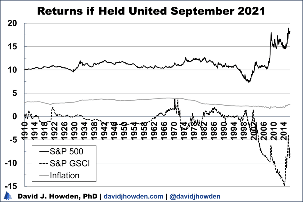
If you bought the S&P 500 in January 1910 and held it until the end of August 2021, you would have realized an annualized total return of 10.0%. (Since we´re looking at a holding period of 121.5 years, each dollar you invested would have grown to $107,000. Your grandkids or great-grandkids would love you.)
If you bought a broad-based basket of commodities in 1910 and held it until today you would have earned 0.6% annually. Inflation doesn´t matter much in this example since it will affect both returns equally, but we can consider it anyway. Since annual inflation has averaged 3.0% in the United States since 1910 you would have lost capital over this looong investment term if you were invested in commodities, but still came out ahead by a sizeable margin if you had bet on stocks.
Let´s pick a different point. The crash of 1929 is etched in many people´s minds. That year the stock market peaked on a monthly closing basis in August. The fool who bought stocks that month was underwater for a long time, but he would be able to realize a total return of 9.6% annually if he held until today.
By way of contrast, if the investor had been smart enough to get out of stocks in 1929 and invested in commodities, on balance his return until today would have been a touch below breakeven. Since inflation has averaged 3.0% since August 1929, again we see that the investment in commodities resulted in a real capital loss to the investor, while the equity investor still came out ahead.
One last example. The market peak in August 2000 was surely a terrible time to invest in the stock market, right? The question is actually difficult to answer because you need to look at what else the investor could have done with his money instead of buying stocks.
If you bought the S&P 500 in August 2000 and held it until today you would be sitting on a respectable 7.4% return, annualized over these 21 years. If you instead bought commodities with that money, you´d be sitting on an annual loss of 2.8% until today. If you held cash, you would have lost 2.2% annually since that is the rate of inflation averaged over the period.
This exercise should reinforce in your mind that stocks are a much better and dependable bet than commodities over looong periods of time. This conclusion is the same as I made in the previous post, but here I have made the case without arbitrarily picking an investment time horizon.
We can simplify the previous chart by considering the excess return from holding equities over commodities. We already know that equities outperformed commodities over all holding periods, but the question of interest is by how much.
In the following chart, we quantify the difference in returns. I´ve truncated the excess return axis at 16% because, with the stock market having an extreme bull market over the last year, the short-term excess return is unusually high. We´ll focus instead on the more “normal” state of affairs. Throughout its history, the S&P 500 has outperformed commodities by about 12% annually.
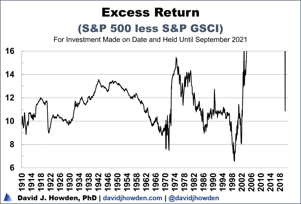
If you bought the stock index in 1910 you earned 10.0% until today against an annual return of 0.6% for the commodity index. This difference amounts to an excess return on stocks of 9.4% annually.
If you bought the S&P 500 in August 1929 you earned an excess return of 9.7% annually over commodities. Even if you bought in 2000 at the stock market peak, you still earned an excess return of 10.2% if held until today.
My goal here is to underscore how normal it is for stocks to beat out commodities. You might quibble that the record highs in the stock market skew the results at the moment. Outside of a few specific resources (like coal), commodity prices in general are still quite depressed. I´ll address this point in a follow-up post where we´ll see that this changes the size of the benefit of stocks over commodities, but not the message.
I emphasize the looong aspect of these periods because, at best, the investor has twenty to forty years to maximize his investment return. Over some shorter periods, stocks have been a worse investment than commodities. Put another way, holding commodities over some shorter periods gives the investor a clear edge in the market. The trick lies in identifying when the stock market is overvalued relative to the commodity market.
One common method to view this relative valuation is by taking the ratio of the two assets. In the chart below I have divided the S&P 500 index by the S&P GS Commodity Index. At the end of August, the S&P 500 closed at $4,522 while the commodity index closed at a price of $527 meaning that the stock market was trading at a multiple of 8.6 times the commodity index.
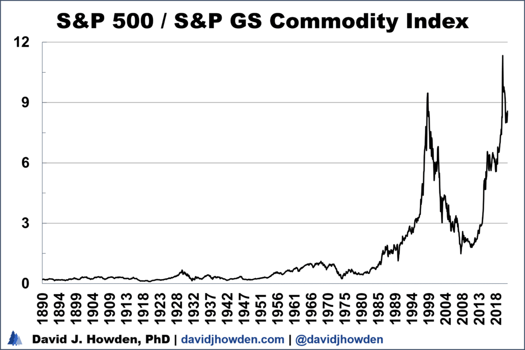
At stock market peaks you expect this ratio to peak also. That´s helpful to know in retrospect, but the challenge is in knowing whether the ratio has already peaked.
Take September 1968, for example. This was close to a major peak in equities, and the S&P 500-to-S&P GS Commodity Index ratio peaked at 1.05. Fast forward to June 1985 when the ratio surpassed this value for the first time. It might have been attractive at that time to think that the ratio had peaked in 1985 since it was at its highest level in seventeen years. Of course with the benefit of hindsight, we know that 1985 was not anywhere near to a stock market top. It was not a top in absolute terms, since the market continued to climb uninterrupted for another decade-and-a-half. And not relative to commodities since it would not be until February 1999 before the S&P 500 peaked against the commodity index.
If the ratio of the two indexes is useful it is in a retrospective way by allowing us to confirm the peaks and troughs in one market relative to another. Of course, we don´t need to take the ratio to see this as we can glean this information, more or less, by looking at each index independently. (We know that 1968 was a major peak for equities, and we know that 1999 was a major low in commodities.)
I have pioneered an approach to look at value in a way that is consistent and normalized over time by way of what I call relative valuation. Relative value looks at how cheap or dear an asset is relative to not just one good but relative to a basket of goods. The components include many of the significant alternative outlays that an investor could make instead of his investment, like food, gas, housing, and many others.
The use of a basket of goods makes it a more general approach to looking at value. In this way, it is similar to other valuation approaches, like the Dow-to-gold ratio or using P/E ratios to signal over or undervaluation in the stock market. It is a superior approach because there are reasons why an individual asset´s price might change relative to a financial asset (interest rates drive P/E ratios; tax treatment or laws drive gold prices) but a broader basket evades these challenges.
I normalize this relative valuation measure over time by expressing it as a statistical z-score. In brief, a z-score is the number of standard deviations an observation is away from the mean. In this case, we can consider the mean to be the “fair” value price of an asset, and the relative valuation to be the number of standard deviations away from that fair-value level it is currently trading at.
Normalizing relative value in this way has some advantages. The first is that it shows us when an asset is over or undervalued relative to its historical norms. Furthermore, it shows us the size of this valuation. And since the measure is, by definition, mean-reverting, we can see the peaks and troughs in the market , something not possible by looking at the asset´s price independently.
Below is a chart showing the valuation of the S&P 500 relative to the S&P GS Commodity Index since 1910. The peaks and troughs are identifiable. The mean-reverting nature of the measure is important since we can see that troughs generally happen around a value of -1, or one standard deviation below the mean. Peaks occur when the S&P 500 is overvalued by 1.5 to 2 standard deviations (or more) relative to the commodity index.
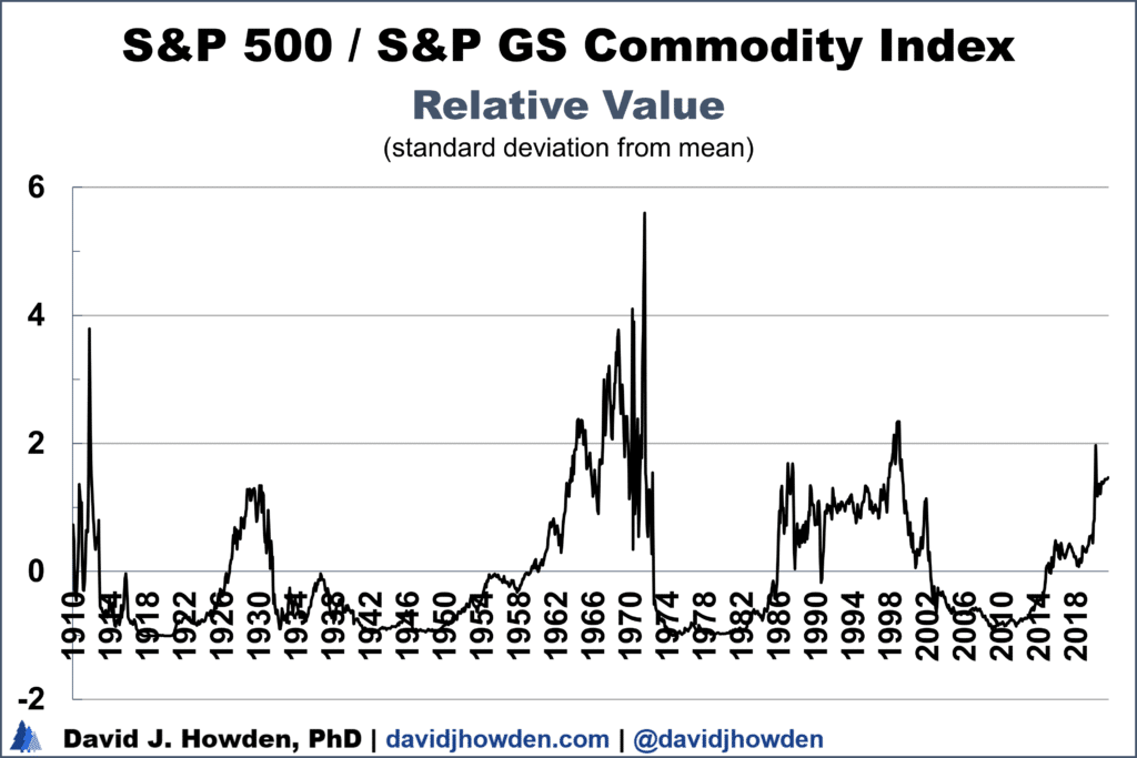
In September 1974 the S&P 500 peaked relative to the S&P GS Commodity Index at a relative valuation of 5.6 standard deviations. This “5-sigma” event is definitely rare, and we can quantify how rare. One of the nice attributes of relative valuation is not that it is mean-reverting over time (with a mean valuation of 0, which is the fair value of the asset) but also that it is normally distributed. (Statistically, the relative valuation of an asset has a mean of zero and a standard deviation of one.) This means that we can easily compute the likelihood of an event occurring.
September 1974 was the most expensive month since 1910 for equities relative to commodities. Of course, the history of stock and commodity markets extends much further back in time than 1910, it´s just that our data series begins there. Taken as a whole, a 5.6 standard deviation overvaluation made the stock market more expensive than commodities in over 99.999997% of its history. Armed with this information, the investor would not bet that stocks were going to become even more highly valued than commodities going forward!
In my previous post, I included a graph of the valuation of the S&P 500 relative to the S&P GS Commodity Index expressed as a percentile. I did this because it is easier for the average person to interpret a percentile than a standard deviation. The investor would understand what it means if I told him that the stock market was more overvalued than essentially all of its history (or 99.999997% of it) in September 1974 than if I told him that it was overvalued by 5.6 standard deviations. Of course, the two ways to express relative value are the same, but one is easier to understand for the layman.
Still, it is helpful to illustrate relative valuation as a standard deviation from the mean for several reasons.
The most important one is that it is hard to tell the difference between the extreme valuations when expressed in percentile form. All z-scores above 2.35 (i.e., anything greater than a 2.35 sigma event) will be in the 99th percentile. This is because the likelihood of occurrence is normally distributed. In valuation terms, there is a big difference between the market being 2.5 versus 5.0 standard deviations overvalued. It is not possible to see this valuation difference on a graph expressed as a percentile.
Statistically, we could say that there is a linear relationship between valuation when it is expressed as a standard deviation, but there is a nonlinear relationship between these valuations when expressed as percentiles. Being overvalued by two standard deviations is twice as overvalued as being overvalued by one. A 1-sigma valuation is more overvalued than 84% of its history, and a 2-sigma valuation more than 97% of its history, meaning the increase in the overvaluation of only 15% (13%/84%). (Actually, that is a convenient way to express the difference but not entirely accurate. The increase means that the market is more overvalued than an additional 13% of its history.)
Having a linear relationship between relative valuations is important because returns relate to each other linearly. Earning 10% is twice the return of 5% on an asset, for example. Having an excess return of 4% on the stock market over the commodity market is half that of earning an excess return of 8%.
Let´s put it all together. We know that stocks are, in general, a better bet than commodities over long investment horizons. But we know also, from the previous post, that there are many examples of shorter investment horizons, less than ten years, where commodities outperformed stocks by a hefty margin. The key to maximizing your investment return is discerning the periods of positive excess stock returns from the negative ones.
The easiest and most dependable method to separate the periods of positive from negative excess returns from an equity investment relative to commodity investments is by looking at the relative valuation at the start of the investment period. Periods when the S&P 500 was overvalued against the S&P GS Commodity Index (signaled by a positive relative valuation) resulted in lower future excess equity returns. The greater the overvaluation, the smaller (or negative) the resultant excess equity return was.
The relationship between the excess return of the stock market over the commodity market and its relative valuation is strong, and clearly negative. Below I´ve plotted the two variables against one another. On the x-axis are the values of the excess return one would earn over a ten-year period by investing in the S&P 500 instead of the S&P GS Commodity Index. On the y-axis I plot the relative valuation at the start of all these ten-year periods, expressed as a standard deviation from the mean.
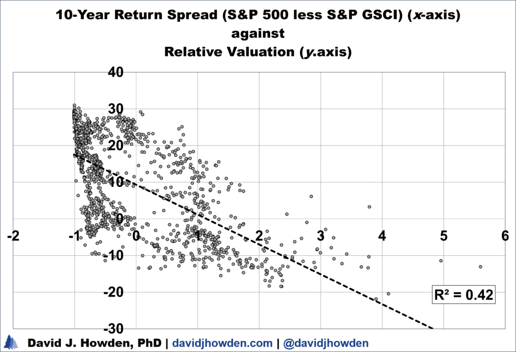
Eyeballing the data we can see the negative relationship. Since the two data series are linearly related, we can also quantify the relationship.
The dotted line of best fit confirms our eyeballing of the data´s negative relationship. (This line is constructed so that the number of points above and below the line is about equal (and the line passes through as many points as possible). The R2 of this line of best fit is 0.42, meaning that relative valuation of the market at the beginning of the period explains 42% of the variance of the 10-year excess return.
It´s not a perfect measure. For starters, we can see a large congregation of points around -1 on the x-axis. This is because the bear markets in the S&P 500 almost never lower its valuation below that level, while bull markets in equities can run to quite extreme highs.
Still, with half of the return variance explained by relative valuation we have the basis of a high-quality model with predictive capability. The predictive capability comes from the fact that although the excess equity return over the next decade will not be known until September 2031, we know today what the relative valuation of the stock market is relative to commodities.
The S&P 500 is overvalued relative to the S&P GS Commodity Index by 1.5 standard deviations. This means that equities are more highly valued relative to commodities than in 93% of their history.
This overvaluation is down somewhat from its high set in April 2020. That month didn´t seem to have especially high valuations in equities, but keep in mind that commodities were especially depressed in early 2020. (Crude oil futures traded at a negative price for a short stint.)
The last time equity valuations came down from their highs and declined to an overvaluation of 1.5 standard deviations was June 1999. Over the next decade, commodities outperformed equities by 14.1% annually. 1999 was the start of one of the greatest commodity bull markets on record, and also the start of one of the most devastating bear markets in equities with the dot-com bust. The time before that was October 1971. The S&P GS Commodity Index outperformed the stock market by 2.3% over the following decade. (In the shorter term, commodities quadrupled in price by 1973, while equities remained flat.)
While looking at specific cases with similar valuations is instructive, we can also statistically test the relationship between relative valuation and subsequent return to see the magnitude of the relationship. (Also we can test for the direction of the relationship, but we already know the two variables are negatively related by eyeballing the scatter chart from before.)
Below is a chart that shows the historical excess returns of equities over commodities for the 1,220 ten-year periods between January 1910 and August 2021. The dotted line shows the best-fit line given the relationship between the starting relative valuation and the subsequent excess return in these cases.
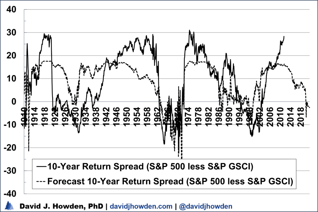
The statistical analysis tells us that there is a baseline excess return from equities over commodities when the market is fairly valued of 9.3% annually. It also tells us that each standard deviation of overvaluation in the S&P 500 against the S&P GS Commodity Index lowers the future excess return by 8.2%.
Given the overvaluation in the equity market of 1.5 standard deviations, the model forecasts that commodities will outperform equities by 2031 by 2.6% annually.
We can see some periods where the model performed less well in explaining the excess return to equities. For the most part, it underestimated the excess return in the 1950s and overestimated it during the latter half of the 1920s. These are important points to keep in mind, but what is more interesting is how the model performs not during equity undervaluations but during overvaluations, as is the case today. Here the model performs quite well. It pinpoints all the periods when commodities outperformed stocks and got the magnitude correct in nearly all the cases also.
The model explains 42% of the variance in equity excess returns. We could improve on this by including more instrumental variables. I do so in my books, and the result is an increase in model accuracy. In this post, I want to focus on the role of relative valuation in isolation of other variables so the reader can get a feel for how important this one variable is in determining future returns.
Every investor knows that the key to superior returns is to buy low and sell high. Relative valuation allows him to have a measure in real-time to signal whether an asset is priced “low” or “high” and by how much.
Conclusion: stocks for the long run, but if you want to maximize your return, commodities for the medium run. Avoiding periods when equities underperform commodities is essential to maximizing your portfolio´s return. Statistically, now is one time where there is good reason to believe that commodities will outperform stocks for the next decade.
One final thought. In my Almanac of Global Equities: 2021-31 I provide more detailed and higher-quality forecasts of thirty-seven of the world´s largest stock markets. Over the next decade, I forecast that the S&P 500 will decline by 2.6% annually (the forecast model in that book incorporates more instrumental variables than the relative valuation of the market, and it explains over 90% of the index´s returns over its ten-year investment periods).
In my book, Commodities, the Decade Ahead, I provide forecasts of forty-three of the world´s major commodities and commodity indexes. By August 2031 I expect the S&P GS Commodity Index to increase in value by 9.6% annually. Again, since the forecasting model I use in my books is superior to this simple example, it can explain a greater amount of the historical returns. The available data explain a full 79% of the commodity index´s ten-year returns.
Taken together, combining these two higher quality forecast estimates commodities outperforming equities by 12.2% annually over the next decade, versus 2.6% in this simple analysis. The important aspect of the analysis is not the exact number, although that is also of interest, but the direction of the trend which is consistent under both approaches.
Using two separate analyses we have drawn the same conclusion: commodities are set to outperform equities over the next decade, and by a sizeable margin. Note that this is a relative analysis. The stock market could still head to new record highs, but it is set to decline relative to commodities. Get your portfolio in order to position yourself for the trend before it takes off.