Consumers, producers, and investors have traded gold since antiquity. Because of the longevity of its use as money, we know the price of gold further into the past than any other good. We usually understand the meaning of a price by looking at its evolution over time. For example, first-year economics students absorb the importance of relative scarcity in determining prices. Increasing prices denote heightened scarcity. Lower prices signal greater abundance.
Like many concepts in economics, the relationship between scarcity and price sounds good from a theoretical perspective. The more pressing issue is how one can use it from a practical point of view.
Gold is an interesting case since its price history extends far into the past. For most of its history before the late 1960s, however, its price was constant.
Consider the following chart. Here we see the price of gold in terms of US dollars since 1791. For most of this period until the end of the gold standard, a slug of the yellow metal defined the value of the dollar, as was the case for most major currencies.
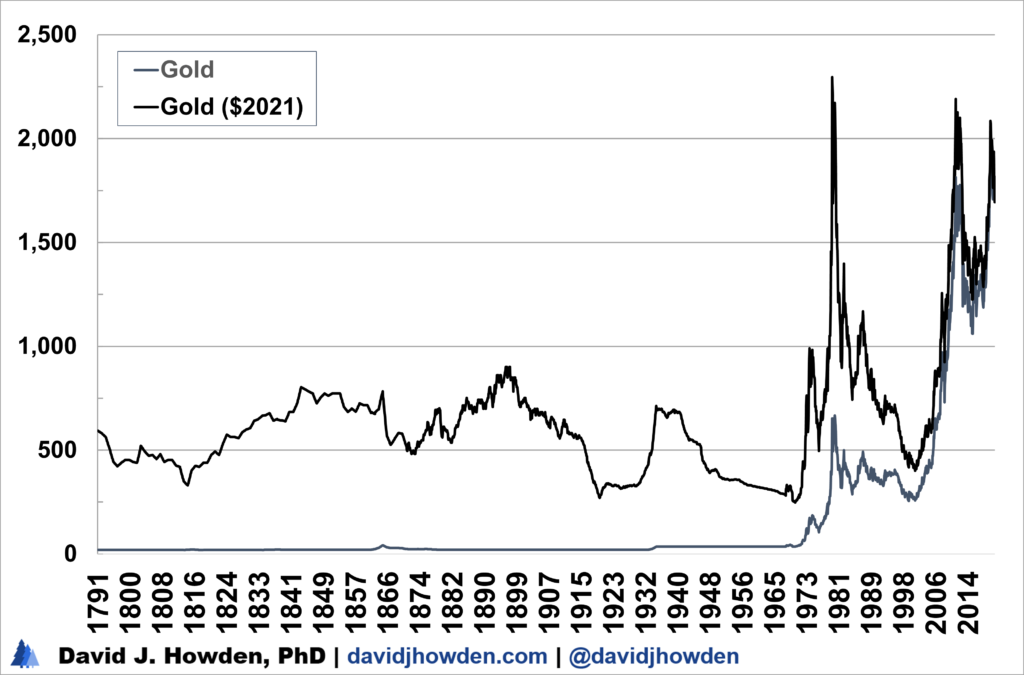
The stability of the gold standard brought very little variance to the price of gold. (Or, more correctly, it brought stability to the dollar.) Until 1934 the value of gold didn´t veer far from the price of $20 an ounce.
The two World Wars interrupted the gold standard, but it resumed under the Bretton Woods system between 1944 and 1973. The US dollar fixed the price of gold under this system, creeping towards flexibility starting in 1968. Since being released from its role in defining the exchange value of the US dollar, gold´s price has skyrocketed.
Some earnest first-year economics students could take the stability in the price of gold before the late 1960s to mean that there was no change in its relative scarcity over the period. Of course, the gold rushes and turmoil over the period did indeed cause significant changes to the metal´s scarcity. This fact is difficult to see by way of gold´s nominal price history.
One way to get a better feel for the value of gold over this period is to focus on its inflation-adjusted price. Doing so brings several advantages. The first is that we can compare a real price from the past with the price today by adjusting it for changes in purchasing power. More to the point, we can see changes in relative scarcity by focusing on changes to the inflation-adjusted price.
I´ve expressed gold´s price in 2021 dollars in the chart so that we can compare its value directly to its price today. Here we see general changes to the relative scarcity of the metal creating several significant bull and bear markets.
From 1814 to 1845, for example, the real price of gold advanced from $336 to $789 while the nominal price did not change. The volatility in the real price during periods like this, when gold´s nominal price was fixed, is of interest to us.
This analysis is interesting from a historical perspective in that it lets us see some of the vicissitudes of the gold market during a bygone era. It is difficult to understand what the value of gold really was during these periods. Even though we´ve adjusted the price to counter the effects of inflation, the only information we have is what the price “feels” like with today´s purchasing power of money. It´s a start, but using real prices falls short of allowing us to understand when gold was cheap and when it was dear.
To shed light on this problem, we can turn to a measure I have pioneered called “relative valuation.” This measure tells us, on average, how expensive or cheap an asset is relative to other prices at a certain time. In this way, we can directly compare prices from the past with those of today. This gives us a sense not only of what period was better valued, but by how much.
There are two ways to think of relative value. The first is as a normalized z-score. Here the value is measured in terms of standard deviations from its mean value. You can think of the mean value as the “fair” value price of an asset at a given time. Since fair value is an ambiguous and confusing term, I will qualify it. It means the valuation relative to other prices which prevailed on average over the good´s history.
An ounce of gold has always sold at a higher price than an ounce of silver. It foreseeably always will, given the relative scarcities of both metals. To say that gold is more expensive than silver today since its price is 77 times higher is true, but not informative. A higher gold price today does not mean the yellow metal is more expensive than silver. A higher, or more expensive price of gold, is the normal relationship between the two prices.
One could look at the gold-to-silver ratio over time and try to glean insight into whether gold is more expensive relative to silver today, and if so by how much. This approach to the problem is also lacking. The factors that determine the prices of gold and silver are distinct. They boil down to specific supply and demand conditions. There is no reason that the ratio of these two prices should be mean-reverting or oscillate around a specific value over time. The ratio might be increasing or decreasing, but that could be due to a change in the scarcity of gold over silver.
Relative valuation solves this problem. Instead of looking at one good´s price relative to another, it looks at the price relative to a broader basket of goods. It accounts for the normal spread in value between the basket and the good´s price over time and informs us of when important divergences develop.
Consider the following chart, which illustrates gold´s relative valuation since 1812. It is expressed as a standard deviation. This might not be intuitive to many but has useful properties and important implications.
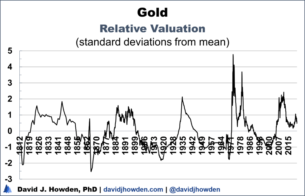
Here we can see the periods when gold was overvalued relative to a broad basket of goods (positive values) and when it was undervalued (negative values). The magnitude of the relative valuation tells us about the valuation in terms of standard deviations (or sigmas).
We know with the benefit of hindsight that gold was trading at a very high price in September 1980. On a monthly closing basis, the metal reached a price of $667 an ounce. This price would not be surpassed until April 2007. In inflation-adjusted terms the metal hit $2,171 in September 1980, higher than ever in its history.
By looking at the nominal price, the investor is unsure of whether gold was selling at a high or low price at the time. We know now that the price collapsed over the following two decades. But at the time, the price was high precisely because so many people thought that gold was cheap relative to the other things they could spend their money on.
Instead of focusing on the nominal price, we could look at the metal´s real, inflation-adjusted price at the time to glean an insight. Here we recognize that gold was trading at a much higher price than ever in its history. But it had a fixed price for almost all its history up to that point. It is difficult to draw conclusions about its valuation based on two very different price regimes. Furthermore, even if we looked at the high real price in 1980 it is very difficult to answer the question of “how much more expensive gold is today than at other periods.” This is because there are many reasons why gold´s real price will differ over time relative to other goods. Again, supply and demand conditions in the local market are important for its valuation relative to other goods.
Now consider the relative valuation chart with the value expressed as a standard deviation from the mean. In June 1980 we find that gold had a value of 2.4 standard deviations. Instead of telling us that gold was overvalued relative to other goods that month by a percentage amount, the measure tells us how many standard deviations overvalued it was. One of the nice facts of relative values, unlike nominal and real prices, is that they are normally distributed. This means that we can perform statistical analyses on them to glean insights that are not possible by using raw price data.
For starters, we can use the relative valuation expressed as a standard deviation to determine the likelihood of its occurrence. A 2.4 sigma event is rare, occurring only 0.8% of the time. This means that in June 1980, gold was more overvalued than it had been in 99.2% of its history.
You might notice when looking at the chart that September 1980 is not gold´s relative valuation high. The local high proximate to September 1980 was several months earlier. In January of 1980, the measure peaked at 3.7 standard deviations. We can compare these two relative valuations directly. Gold was 54% more highly valued in January than it was in September. You might find this confusing since the nominal price was only 2% higher at the end of September than at the start of the year.
Gold was more expensive in September 1980 than at the start of the year, but so were all prices. Annual inflation was, after all, over 12% in 1980. Gold was actually more overvalued relative to these other goods at the beginning of the year than it had been by September. Relative valuation captures this.
The real price for the metal peaked in January 1980, consistent with the relative valuation top. Considering these dual tops, you might think that using the real price as a signal of overvaluation would be more beneficial. It accomplishes the same goal in a more straightforward way. What relative valuation brings to the table is an ability to tell you the magnitude of the over or undervaluation. Relative to its history, gold was overvalued by 3.7 standard deviations in January 1980. This overvaluation is only likely to occur 0.02% of the time. In other words, gold was more overvalued that month than in 99.98% of its history. Another way to look at this is to say that the nominal gold price was 3.7 standard deviations overvalued.
Looking at the chart you might realize that the all-time relative valuation peak came in May 1973 at a value of 4.8 standard deviations. This implies that gold was valued more highly relative to other goods at that time than in 99.9998% of its history.
May 1973 is not, by all appearances, a significant high. At least, it isn´t in nominal terms. Gold closed the month at $114 an ounce, or a real price of $23.
The reason for the extreme overvaluation is twofold. On the one hand, gold´s price rocketed in a short space of time. It more than trebled over the previous three years. This rapid price spike, the most extreme in 230 years under examination, made the metal expensive relative to other goods in a very short period. The second reason is that while gold´s price was increasing between 1970 and 1973, other prices were not. At least, they were increasing at a much slower rate. Annual inflation in 1973 was still under 4%, while gold´s price increased by 72%. High inflation didn´t come until later in the decade. In 1973, gold was very expensive relative to other goods by its historical norms.
Converting the standard deviation values into percentiles makes it easier to interpret relative valuation. In the graph below I´ve done just that. We can interpret the percentile as the percentage of time that gold was priced at a better value. If gold is valued at the 100th percentile, it is more expensive relative to other goods than it has ever been. If it is in the 0th percentile, it is cheaper than it has ever been. To be valued in the 50th percentile means that the metal is fairly valued. Technically this means that it is at its average valuation relative to the other goods over its history.
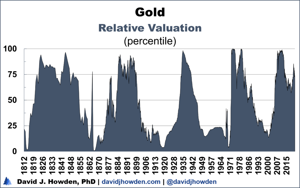
This graph communicates most of the same information as the previous one expressed in standard deviations. It is also easier for the layman to understand.
Gold was valued in the 90th percentile or higher in 1824, 1844, 1886, 1894, 1934, 1973, 1980, and 2010-12. These moments when gold was extremely overvalued relative to other goods provided a clear signal that its price would lag relative to other prices in the future.
Returning to the chart illustrating the real price of gold over time, we find many of these peaks coincide with major tops. 1844, 1894, 1934, 1973, 1980, and 2011 were all noticeable peaks in the precious metal´s inflation-adjusted price. (1824 and 1886 were minor tops.)
What about the bottoms in the metal´s valuation? Gold was valued in the 10th percentile or lower on six occasions: 1815, 1865, 1872, 1910, 1920, and 1970. At the inflation-adjusted bottom in 2001 the metal was valued in the 13th percentile.) Returning to our inflation-adjusted chart, we can see that those were good moments to buy the metal as they represented important major market bottoms.
The terms market top or bottom are convenient, but what we are looking for are those periods that resulted in a superior return to holding gold. Consider the five-year returns in the chart below.
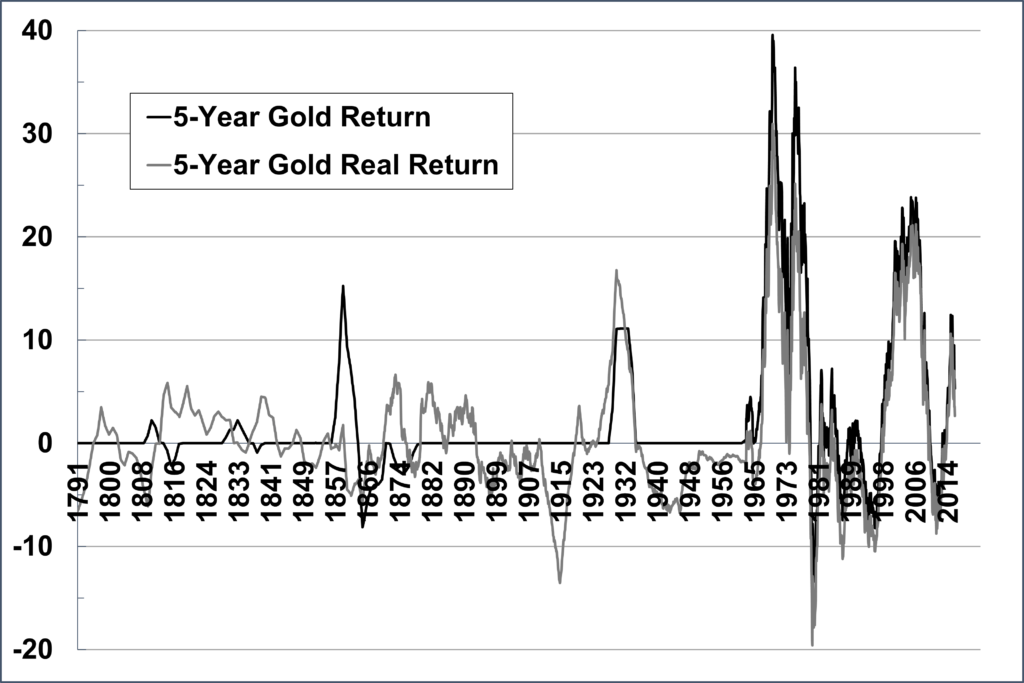
The chart shows the return the investor would earn by buying gold at a certain date and selling five years later. It lets us see exactly how good the investment returns were over this short period of time. I´ve included both the nominal and real returns. The real return is often more illustrative since the nominal return to holding gold has been zero over most of its history. By focusing on the real returns, we revisit some familiar dates.
Buying gold in 1930, 1975, or 2006 all yielded double-digit annual returns to the investor. If you bought gold in 1969 you would have earned an annualized real return of 31% over the next five years.
We also see some periods where the investor did not want to hold gold. Buying the metal in 1915, 1970, 1987, and 1996 all yielded annual losses of more than 10%.
Looking at the vicissitudes of the gold market this way, we see the importance of measuring the value of gold not only by its nominal and real prices, but also by its relative valuation. There is no correlation between gold´s return and its real price. There is a strong correlation between gold´s relative valuation and its future return. The reason is intuitive. When gold is expensive relative to other goods, investors take advantage of this value spread by moving out of gold and into other channels. This starts to depress gold´s price and lowers its future return.
We see this exact scenario playing out time and time again. Buying gold at its peak valuation in May 1973 worked out fine for a short while. Ultimately the investor was underwater on the investment until 1985. That´s a long time to go to secure a real return of zero.
Buying gold when it was overvalued by 3.7 standard deviations in January 1980 resulted in a real loss of 9% annually over the next decade, and 19% annually by 1985.
In August 2011 the metal was overvalued relative to other goods by 2.4 standard deviations. Over the next decade, the investor would have lost 2.5% annually in real terms, and 7.5% annually by 2016.
Gold wasn´t exactly on too many investors’s horizons in 1934. Roosevelt´s Executive Order 6102, signed on April 5, 1933, made it illegal for US citizens to own gold. The prohibition remained until December 31, 1974, when Gerald Ford legalized the private ownership of the metal.
Other than avoiding a prison sentence, there were other good reasons to not want to hold gold in the aftermath of the executive order. By December 1934, gold was overvalued by 2.1 standard deviations. This made it more expensive than 98% of its history. Anyone holding gold on that date lost 3% annually over the next decade, and 1% annually by 1939 in real terms.
So much for investment nightmares in the gold market. Let´s focus on the dreams. We know with the benefit of hindsight that buying gold in 1920, 1970, or 2001 yielded incredible long-term real returns. The problem is that at the time it is difficult to tell good from bad values. Indeed, the reason why gold sold at such great value in those three years is that it was so out of favor. Relative valuation solves this problem.
In June 1920 gold was undervalued by 1.7 standard deviations. This made the metal cheaper than 96% of its history. That turned out to be an incredible time to invest, even though its price was still fixed by law. The nominal return over the next five and ten years was zero. But its real return turned out to be positive. If you bought gold in 1920 and held it until today, you realized a return of 4.5% annually over the 101-year period. Each dollar you invested would now be worth $85, such is the wonder of compounded returns.
It was still illegal for Americans to hold gold in 1970. The Bretton Woods system fixed its price for several decades, and most international investors weren´t too keen to diversify into this untested commodity. Still, if you watched the relative valuation of the metal, you would have realized that by July 1970 gold was valued near record lows. Valued 1.8 standard deviations below its fair value, it was cheaper than in over 96% of its history. Armed with this knowledge, the adventurous investor could have loaded up. His investment would have paid off handsomely. Gold surged to a real return of 23% over the next decade, and 28% annually by 1976.
Gold may have bottomed in nominal terms in 1999, but it kept shedding value until March 2001. That month, undervalued by 1.1 standard deviations, the metal was cheaper than 87% of its history. It had been beat-up over the previous two decades and investors shunned it as an investment. Anyone smart enough to diversify into gold that month would have been rewarded with a real return of 16% over the next decade, and 15% over the next five years.
I could go on, but the reader can pick out other examples from the graphs above.
Gold has been used as money, as a consumer good, and as an investment for thousands of years. We have a longer price history of the metal than any other good. For most of its history, however, its price has been fixed as it was the monetary unit. This makes it difficult to see bull and bear markets as price stability gives the illusion that its value was fixed until the late 1960s when the breakdown of the Bretton Woods system liberalized its price. Adjusting for inflation allows us to see that there were important and significant swings in its real price over time that created attractive investment opportunities. There were also times when it would have been prudent to step back and let the market resolve itself.
Relative valuation is a measure that we can use to determine whether gold (or any financial asset) is over or undervalued relative to other opportunities. Furthermore, it allows us to gauge the magnitude of the over or undervaluation. In real-time, the measure gives us a feel for how prudent it may be to invest in the metal.
Gold is currently overvalued at 0.5 standard deviations. This means that it is more expensive than other goods in more than 68% of its past. As we´ve seen, in the grand history of its bull markets, overvaluations typically move much to much higher valuations than this. Never in the 230-year history under examination has a major bear market in gold started from an overvaluation of less than 1.5 standard deviations. Gold might be far along its way on its current bull market. But if history is any guide, it still has lots of room to stretch its legs.